Prode Properties
Properties of pure fluids and mixtures, multi phase equilibria, process simulation, software
Title : Dew point software cricondentherm natural gas hydrocarbons hydrate formation with Excel Matlab Mathcad software


Contact Prode
Excel / Matlab application example : dew point, bubble point, cricondentherm, cricondenbar, critical point
Prode Properties has specific methods which permit to calculate dew points, bubble points, equilibrium points at specified phase fraction (vapor, liquid, solid **) and pressure (or temperature), typical applications include hydrocarbons dew point (HDP, HCDP), cricondentherm, cricondenbar of natural gas mixtures from gas analysis.
Prode Properties can calculate up to 5 equilibrium points along a line with specified phase fraction, in addition there are specific methods for calculating directly Cricondentherm, CricondenBar and Critical points. With Prode Properties you can do this in Excel, Matlab or any compatible application including custom software, this example shows how to use these methods in Excel.
First step: define the stream (components, compositions etc.)
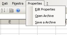
Properties includes a Stream editor which permits to access all informations (as compositions, operating conditions, models, options) for all streams which you need to define, to access the Stream editor from Excel Properties menu select Edit Properties
The Stream editor includes several pages, from the first page you can select a stream (Properties can store all the streams required to define a medium size plant) solve a series of flash operations and see the resulting compositions in the different phases, in this page select the stream you wish to define, for example the first.
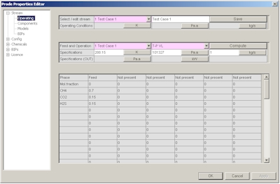
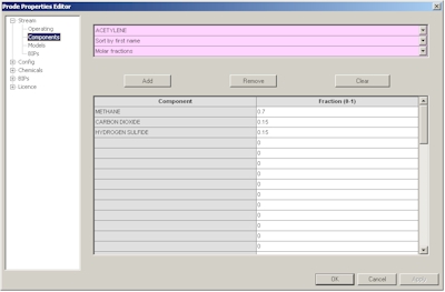
In the second page you can define a new composition or modify an existing composition, in this example we define C1 0.7 CO2 0.15 H2S 0.15 as molar fractions
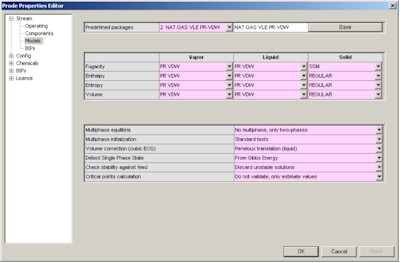
In the third page you can define the package (thermodynamic models and related options) , here we define API Soave Redlick Kwong.
The fourth page provides access to BIP (Binary Interaction Parameters) for the different models, you can enter specific values or click on "Load BIPs" button to get the predefined BIPs from databank.
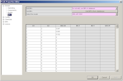
Finally we must save the new data, in the first page click on "Save" button, note that you can redefine the name of the stream as you wish (editing the cell near the button "Save"), you can define / modify many streams following the procedure described.
Once defined the stream you may wish to define the units which we wish to utilize in our problem, in stream editor go then to the "Units" dialog
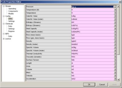
here you can select the units which you need for a specific problem, in this example for the pressure (first row) select Bar.a , notice that unit for temperature is K (but you can set the units which you prefer) then click on Ok button to accept new values and leave the Properties editor.
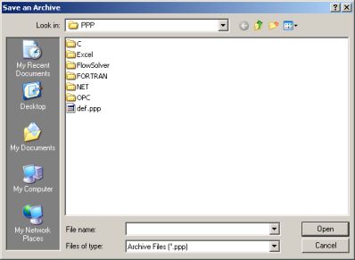
Now you are ready to use Properties for calculating all the properties which you need, however there is still a last thing to do if you do not wish to lose all data when leaving a Excel page, precisely to save data to a file, to save data to a file from Excel Properties menu select "Save a Archive"
then select the file "def.ppp" if you wish that Properties utilizes this data as default (this is the normal , recommended option), differently set a different name (you can for example define different names for different projects) but you will need to load that specific Archive before to make calcs for that project and since Excel reloads Properties with any new page this may result tedious...
Properties saves on the file also the units of measurement so you can define different streams and different units in different projects.
Now you can calculate all the properties which you need with the units which you prefer for all the streams defined in that project.
Second step: calculate properties in Excel cells.
Prode Properties includes methods for calculating critical points and equilibrium points at specified conditions, see the paragraph Methods for thermodynamic calcs in operating manual for the details.
- methods LfPF() and LfTF() are based on a liquid fraction specification, they returns the first point (along the specified liquid fraction line) at the specified pressure (or temperature)
- methods PfPF() and PfTF() can accept a gas, liquid, solid ** fraction as specification, they can calculate up to 5 points (at specified pressure or temperature) along the line with specified phase fraction
- methods StrPc() and StrTc() returns the critical pressure (or temperature) of the nth (from 1 to 5) critical point found.
- methods StrCBp() and StrCBt() returns the pressure (or temperature) of the CricondenBar (the equilibrium point with maximum pressure).
- methods StrCTp() and StrCTt() returns the pressure (or temperature) of the CricondenTherm (the equilibrium point with maximum temperature).
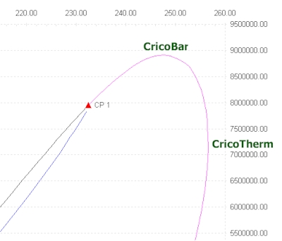
Suppose we wish to calculate a equilibrium point near the critical point for the mixture defined in stream 1, to get the first critical point pressure we enter the macro =StrPc(1,1) where (1,1) refers to the stream 1 and first critical point detected, we enter this macro in B1, in B2 we enter the macro =StrTc(1,1) to calculate the critical temperature in the same way, in cells B3 and B4 we enter the macros = StrCBp(1) for CricodenBar pressure and = StrCTt(1) for CricodenTherm temperature, with this data we have a plot of the whole phase envelope.
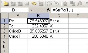
Note that Prode Properties includes methods to plot the phase envelope directly in Excel, go to the page Phase envelope to investigate this option.
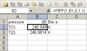
Now we wish to calculate two equilibrium points on the dew line (the red line in phase envelope) at pressure of 89 Bar.a (remember that maximum value is the CricondenBar pressure which is 89.09 Bar.a), we use the method
double t = PfPF(integer stream, double p, double pf, int state, int n)
In cell B1 we define a value for the equilibrium pressure (89 Bar.a) , then in cells B2, B3 we enter the macros
=PfPF(1,B1,0,1,1)
=PfPF(1,B1,0,1,2)
where the first value (1) is the stream , the second (cell B1) represents the pressure, the third (0) is the phase fraction (with 0 we specify 0% liquid or a point on dew line, the same would be by setting the state as gas and phase fraction as 1.0) the fourth (1) is the state (in Properties 0 = gas, 1 = liquid, 2 = solid) and the last is the required position (we require the points 1-2 along the dew line)
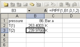
If we change the value of equilibrium pressure the procedure calculates the new equilibrium temperatures
Now a more elaborate example, we define a stream with the mixture Methane 0.999 n-Butane 0.001
- from Properties menu select Edit Properties
- in Stream->Operating dialog we select the stream number 2 and define the name ?Mixture 2?
- then we select Stream->Components dialog and define a composition of two components with following molar fractions Methane 0.999 n-Butane 0.001
- in Stream->Models dialog we define the Peng Robinson (PR-VDW) for all properties
- then we can edit BIPs, we can input data or load from database
- in Stream->Operating dialog we click on Save button to save the stream data
- Now the stream 2 has been defined
The phase envelope for this mixture shows up to four saturation point pressures at the same temperature
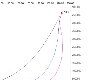
Observe the dew line, the red line below the critical point, there are up to three different equilibrium points at the same temperature (the area around 190 K), if you add the saturation point on the bubble line (black line) we have a total of four saturation point pressures at a given temperature, to calculate the points on the dew line we use the method:
double p = PfTF(integer stream, double t, double pf, int state, int n)
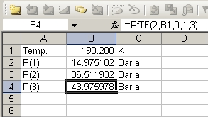
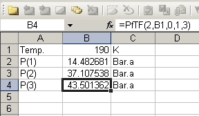
In cell B1 we define a value for the equilibrium temeperature (190.208 K) , then in cells B2, B3, B4 we enter the macros
=PfTF(2,B1,0,1,1)
=PfTF(2,B1,0,1,2)
=PfTF(2,B1,0,1,3)
where the first value (2) is the stream which we defined, the second (cell B1) represents the temperature, the third (0) is the phase fraction (with 0 we specify 0% liquid or a point on dew line, the same would be by setting the state as gas and phase fraction as 1.0) the fourth (1) is the state (in Properties 0 = gas, 1 = liquid, 2 = solid) and the last is the required position (we require the points 1-3 along the dew line)
If we change the temperature the procedure recalculates equilibrium pressures
you may wish to test the method LfTF(), enter the macro
=LfTF(2,B1,0)
where 2 is the stream, B1 represents the temperature and 0 is the (liquid) phase fraction, notice that you?ll get the same values as for the first equilibrium point in PfTF(), by changing the specification we can use the method LfTF() to calculate the point on bubble line
=LfTF(2,B1,1)
where 1 is the specification (100% liquid) for a point on the bubble line , but of course you get the same result with the method:
=PfTF(2,B1,1,1,1)
where the third value (1) is the phase fraction (with 1 we specify a 100% fraction) the fourth (1) is the state (in Properties 0 = gas, 1 = liquid, 2 = solid) and the last is the required position for the point.
Calculate properties in Matlab.
From Matlab command line you can call the methods in Prode Properties by typing the names, for example to calculate equilibrium temperatures at specified pressures
>> =PfTF(2,190.208,0,1,1)
>> ans = 14.975
>> =PfTF(2,190.208,0,1,2)
>> ans = 36.511
in Matlab (as In Excel) you can access the Properties editor from menu associated with the figure.

Prode Properties, technical features overview (Windows version)
- Entirely written in C++ (since first edition, 1993)
- Up to 100 different streams with up to 50 components per stream (user can redefine)
- Several compilations of chemical data and BIPs are available, the user can add new components and BIPs
- Proprietary compilation with data for more than 1600 chemicals and 30000 BIPs
- flexible database format (support for up to 30 different correlations) works with all majour standards including DIPPR.
- Comprehensive set of thermodynamic models, base version includes
- Regular
- Wilson
- NRTL
- UNIQUAC
- UNIFAC
- Soave-Redlich-Kwong (standard and extended version with parameters calculated for best fitting of vapor pressure, density and enthalpy)
- Peng-Robinson (standard and extended version with parameters calculated for best fitting of vapor pressure, density and enthalpy)
- Benedict Webb Rubin (Starling) BWRS
- Steam Tables IAPWS 95
- ISO 18453 (GERG 2004)
- ISO 20765 (AGA 8 model)
- Lee-Kesler (Plocker) LKP
- CPA Cubic Plus Association (SRK and PR variants)
- Hydrates (Cubic Plus Association, Van Der Waals-Platteeuw)
- additional models as Pitzer, NRTL for electrolyte solutions, PC SAFT (with association), GERG (2008) etc.
- van der Waals and complex mixing rules to combine equations of state with activity models
- Huron Vidal
- Wong Sandler ( WS )
- Michelsen ( MHV2 )
- Tassios et al. ( LCVM )
- Base and Extended EOS versions with parameters calculated to fit experimental data from DIPPR and DDB
- Selectable units of measurement
- Procedure for solving fluid flow including multi phase equilibria and heat transfer
- Procedure for solving staged columns
- Rigorous solution of distillation columns, fractionations, absorbers, strippers...
- Procedure for calculating hydrate formation temperature and hydrate formation pressure
- hydrate phase equilibria based on different Van Der Waals-Platteeuw models
- Procedure for solving polytropic compression with phase equilibria
- Huntington method for gas phase
- Proprietary method for solving a polytropic process with phase equilibria
- Procedure for solving isentropic nozzle (safety, relief valve with single and two phase flow)
- HEM, Homogeneous Equilibrium
- HNE-DS, Homogeneous Non-equilibrium
- NHNE, Non-homogeneous Non-equilibrium
- Procedure for simulating fluid flow in piping (pipelines) with heat transfer
- Beggs and Brill and proprietary methods for single phase and multiphase fluid flow with heat transfer
- Procedure for fitting BIP to measured VLE / LLE / SLE data points (data regression)
- Procedure for fitting BIP to VLE values calculated with UNIFAC
- Functions for simulating operating blocks (mixer, gas separator, liquid separator) **
- Functions for accessing component data in database (the user can define mixing rules)
- gas / vapor-liquid-solid fugacity plus derivatives vs. temperature pressure composition
- gas / vapor-liquid-solid enthalpy plus derivatives vs. temperature pressure composition
- gas / vapor-liquid-solid entropy plus derivatives vs. temperature pressure composition
- gas / vapor-liquid-solid molar volume plus derivatives vs. temperature pressure composition
- Flash at Bubble and Dew point specifications and P (or T)
- Flash at given temperature (T) and pressure (P) multiphase vapor-liquid-solid, isothermal flash
- Flash at given phase fraction and P (or T), solves up to 5 different points
- Flash at given enthalpy (H) and P multiphase vapor-liquid-solid, includes adiabatic flash
- Flash at given enthalpy (H) and T multiphase vapor-liquid-solid, includes adiabatic flash
- Flash at given entropy (S) and P multiphase vapor-liquid-solid, includes isentropic flash
- Flash at given entropy (S) and T multiphase vapor-liquid-solid, includes isentropic flash
- Flash at given volume (V) and P multiphase vapor-liquid-solid, includes isochoric flash
- Flash at given volume (V) and T multiphase vapor-liquid-solid, includes isochoric flash
- Flash at given volume (V) and enthalpy (H) multiphase vapor-liquid-solid
- Flash at given volume (V) and entropy (S) multiphase vapor-liquid-solid
- Flash at given enthalpy (H) and entropy (S) multiphase vapor-liquid-solid
- Rigorous (True) critical point plus Cricondentherm and Cricondenbar
- Complete set of properties for different states
- gas density
- vapor density
- liquid density
- solid density
- gas Isobaric specific heat (Cp)
- vapor Isobaric specific heat (Cp)
- liquid Isobaric specific heat (Cp)
- gas Isochoric specific heat (Cv)
- vapor Isochoric specific heat (Cv)
- liquid Isochoric specific heat (Cv)
- gas cp/cv
- liquid cp/cv
- Gas heating value
- Gas Wobbe index
- Gas Specific gravity
- gas Joule Thomson coefficients
- vapor Joule Thomson coefficients
- liquid Joule Thomson coefficients
- gas Isothermal compressibility
- vapor Isothermal compressibility
- liquid Isothermal compressibility
- gas Volumetric expansivity
- vapor Volumetric expansivity
- liquid Volumetric expansivity
- gas Speed of sound
- vapor Speed of sound
- liquid Speed of sound
- vapor + liquid (HEM) Speed of sound
- gas Viscosity
- vapor Viscosity
- liquid Viscosity
- gas Thermal conductivity
- vapor Thermal conductivity
- liquid Thermal conductivity
- gas compressibility factor
- vapor compressibility factor
- liquid Surface tension
Typical applications
- Fluid properties in Excel, Matlab, Mathcad and other Windows and UNIX (**) applications
- Thermodynamics, physical, thermophysical properties
- Process simulation
- Heat / Material Balance
- Process Control
- Process Optimization
- Equipments Design
- Separations
- Instruments Design
- Realtime applications
- petroleum refining, natural gas, hydrocarbon, chemical, petrochemical, pharmaceutical, air conditioning, energy, mechanical industry